I started writing about coffee prices kind of on a whim—mostly because I wanted to try out this tool called quarto that I’d heard good things about. At the same time, I was curious to see how useful ChatGPT would be when dealing with tabular data, since most of the hype is around text and image/video stuff.
Along the way, I ended up realizing just how much the open source community has given to the data science world—there’s a ton of amazing tools out there. For most projects, I’ve found that the bulk of my time goes into exploring the data and evaluating different ways to frame the problem. Trying out different approaches and prepping the data for each one—that’s what really eats up modeling time.
I’m not really in the “one model to rule them all” camp—first it was deep learning, now it’s generative AI. I’m definitely curious to see what gen AI can do, but I’m keeping a healthy dose of skepticism.
Anyway, while I was digging into all this, I stumbled across some pretty neat libraries—no regrets. One of them was hmmlearn, which is great for working with Hidden Markov Models. This post is really just me wrapping up what I started—gotta close the loop!
Here’s a brief recap of the story so far: we can use time series decomposition to break down the coffee price data into three main components — trend-cycle, seasonal, and noise.
It’s worth noting that people often confuse cycles with seasonality. The key difference is that cycles don’t follow a fixed or precisely defined period, whereas seasonal patterns do. For example, a weekly seasonal pattern repeats exactly every week.
This distinction is why some authors — such as Hyndman (Hyndman and Athanasopoulos 2018) — prefer the term trend-cycle instead of simply trend. The decomposition process typically captures both long-term trends and irregular cycles as a single trend-cycle component. In contrast, the seasonal component represents consistent, repeating patterns and is treated separately.
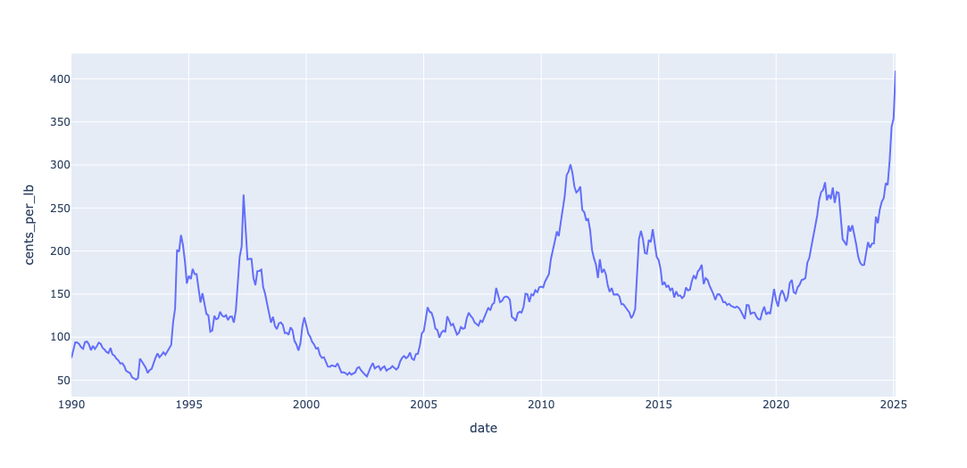
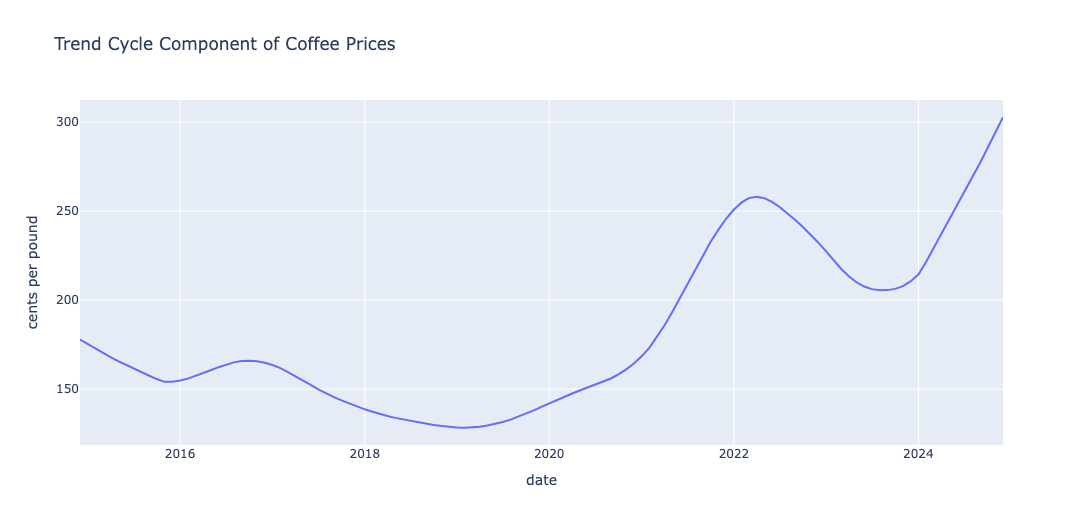
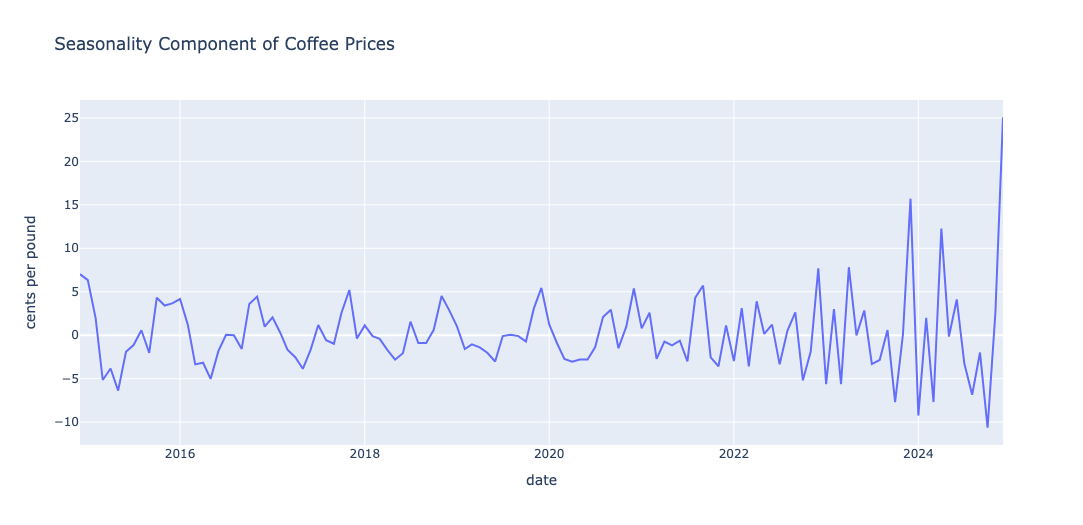
The decomposition of the coffee time series using LOESS(Cleveland et al. 1990) is shown in the panel above. A review of the trend-cycle component reveals approximately \(4\) major cycles. The seasonal component reflects noticeable shifts beginning around 2022, likely due to the impact of COVID. I was able to identify at least \(3\) distinct seasonal patterns during the period.
Altogether, this led me to expect around \(7\) significant changes in the series — \(4\) from the trend-cycle and \(3\)–\(4\) from seasonal variations — dating back to the start of the series in 1990.
One of the benefits of analysis prior to model building is that we get to understand the components that account for the variation in the data. A review of the plots for trend-cycle and seasonality shows that the trend-cycle component is what accounts for the majority of the variation in prices.
If you’re a commodities pricing expert and you see additional changes beyond these, I’d be very interested in learning more about your interpretation.
The residuals — the remaining variation after removing both trend and seasonal effects — are shown in the panel below.

Running change point analysis gave us the changepoints represented in the series below
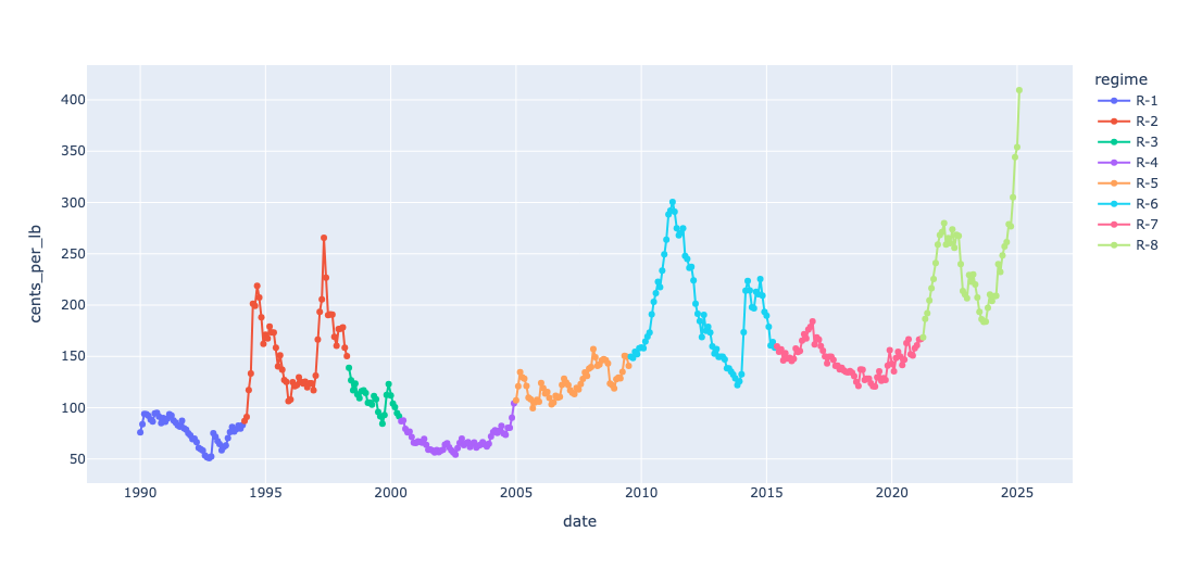
In the previous post, I mentioned that Markov Models are powerful tools for modeling stochastic processes. By discretizing regime prices into three levels — (low, medium, high) — we can apply the theory of Markov chains to estimate the probability of being in each state, known as the stationary probability.
In this post, I’d like to complete the loop by introducing a practical extension for monitoring sequential data like this: the Hidden Markov Model.
Instead of discretizing prices into fixed categories like (low, medium, high), we can let the data guide the analysis using a kernel density estimator (or a histogram — here, I’ve used a KDE). In other words, the discretization is data-driven rather than predefined.
This analysis focuses on Regime 8, which corresponds to the current period in coffee prices. A kernel density plot of these prices is shown below.
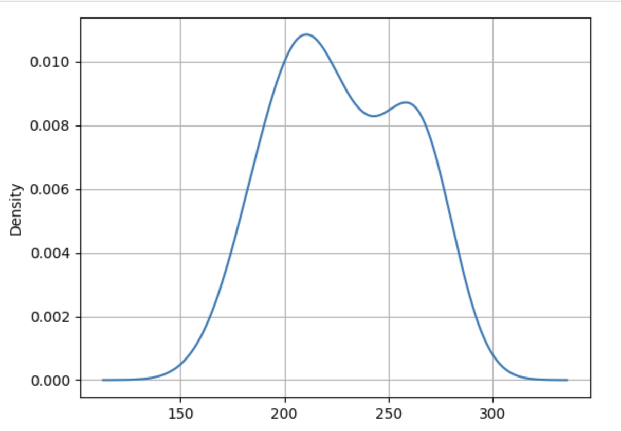
A look at the KDE above reveals that coffee prices tend to concentrate around specific values. In this case, the distribution appears bi-modal — suggesting two distinct clusters of prices. Rather than arbitrarily discretizing prices into three levels, it’s more effective to first histogram the data and then estimate the number of underlying components.
What we uncover here is a 2-state Hidden Markov Model. Coffee prices are clustering around two primary levels, but the cluster membership is latent — we don’t observe it directly. Instead, what we observe at each time step is a noisy sample from one of these clusters.
You can think of this like monitoring patients in a hospital ward where only two health conditions are possible: condition A or condition B. As a healthcare worker doing daily rounds, you don’t get to see a label revealing a patient’s condition — instead, you observe noisy indicators like temperature and vital signs, and from those, you infer the likely condition.
Similarly, each month we observe a single coffee price reported by the time series publisher. Based on that value — a noisy sample — we can infer which price cluster (or state) the market is in.
I’m not going into the details of how the Hidden Markov Model is estimated from the data here. For that, I referred to Bishop’s book (Bishop 2006), which offers a solid conceptual introduction. For those eager to dive deeper, I recommend (Rabiner 1989) and (Bilmes et al. 1998).
By the way, if you’re interested in Graphical Models, Bishop’s book and Jeff Bilmes’ lecture series on YouTube are both excellent resources.
The HMM model estimates these two clusters for us. The kernel density estimates are shown below
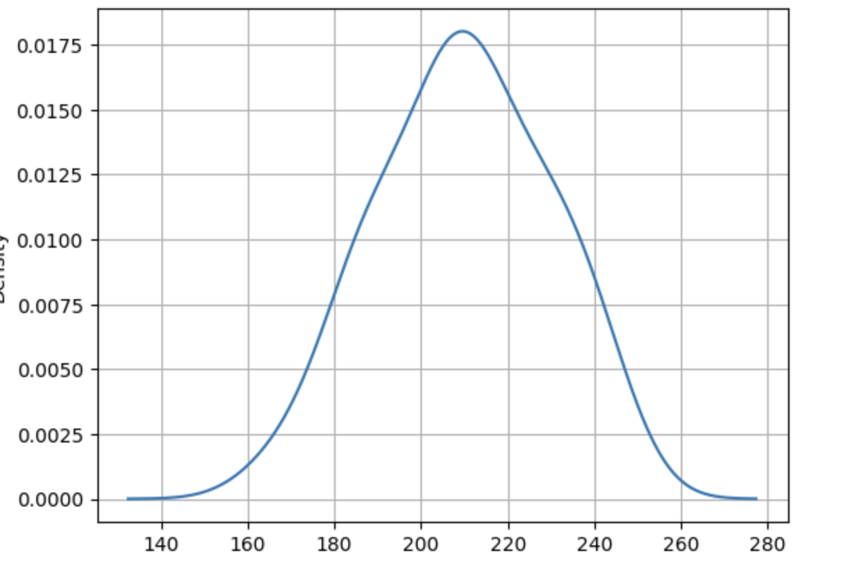
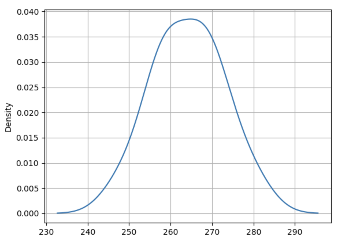
The density plots reveal that cluster 0 is characterized by a lower mean and higher variance, while cluster 1 has a higher mean and lower variance.
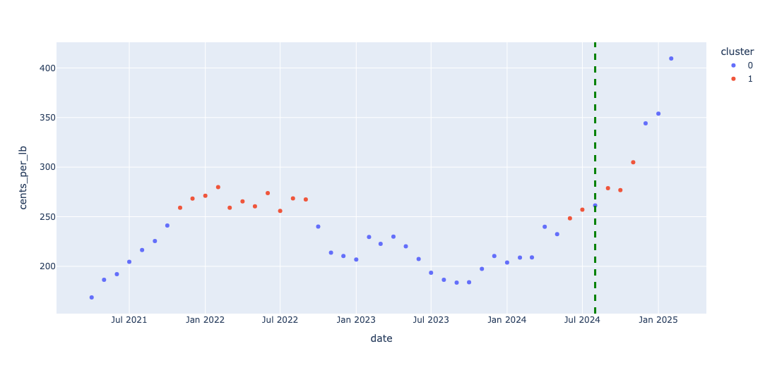
In total, there are \(47\) data points in the current regime (Regime 8). The first \(40\) points were used to estimate the Hidden Markov Model, and the fitted model was then applied to predict the cluster membership for the remaining \(7\) data points.
This is illustrated in the figure below.
While Hidden Markov Models may not be state-of-the-art for prediction tasks, they remain incredibly useful for monitoring and understanding the underlying structure of a time series. Personally, I believe the insights they offer make them well worth the time investment.
That’s a wrap on the coffee prices series — thanks for following along!
References
Citation
@online{sambasivan2025,
  author = {Sambasivan, Rajiv},
  title = {Using {Hidden} {Markov} {Models} with the {Coffee} {Prices}
    {Data}},
  date = {2025-04-26},
  url = {https://rajivsam.github.io/r2ds-blog/posts/markov_analysis_coffee_prices/},
  langid = {en}
}